Dynamical Systems
A dynamical system means that two or more things interact with
each other, resulting in time-dependent behaviour of the whole. If
the interaction has a continuous character and can be expressed using
differential equations, then powerful computational techniques for
differential equations become applicable. For this reason, most
dynamical systems that people study involve systems of differential
equations. We now study some interesting examples.
Predators and Prey
Perhaps the best-known dynamical system in biology is the
Lotka-Volterra model for predator and prey populations.
| dx/dt = x - xy |
| dy/dt = xy - ky |
Here x and y represent prey and predator
populations, and k is a constant. The population
values x=k, y=1 represent an equilibrium or fixed
point. In general, the populations oscillate about this
equilibrium.
The Lotka-Volterra system is often written with four parameters,
rather than just the one parameter k that we have here. We can
insert three more parameters, by multiplying each variable by an
arbitrary constant.
Under this operation, the equations then take the more common
form.
| dX/dT = CX - (BC)XY |
| dY/dT = (AC)XY - CkY |
The extra factors A,B,C are just a matter of units, and
have no effect on the dynamics. In the continuous case of the loops
example C is equal to 0.05, C*B is 0.0002 (B=0.004), A*C is 0.0001
(A=0.002), and C*k was 0.1 (k=2), the unit for T was days and the units
for X and Y were numbers of animals.
Solving differential equations involves replacing the continuous
time variable with discrete time steps. The simplest such
prescription would be
dx_dt = x[i] - x[i]*y[i] #dx_dt stands for dx/dt
dy_dt = x[i]*y[i] - k*y[i] #dy_dt stands for dy/dt
x[i+1] = x[i] + dx_dt*dt
y[i+1] = y[i] + dy_dt*dt
where dt is the discrete stime step. The error is
proportional to dt if dt is small, but if
the time step becomes too large the numerical procedure can become
unstable and give nonsense results.
Write a program to follow the Lotka-Volterra system, and
plot
x and
y against
t, for various different
initial conditions. Then plot
x(
t)
against
y(
t) for several different initial conditions
(but fixed
k) on the same figure. The latter shows an
important qualitative property of the Lotka-Volterra system.
Submit the program
Library solvers for ODEs
This part is optional.
Having the error proportional to the timestep is very inefficient.
A better algorithm can make the error proportional to a higher power
of the timestep. (That power is known as the order of the method.)
Sophisticated algorithms can also guard against numerical
instabilities. The library
function scipy.integrate.odeint() provides an
implementation of the best known general-purpose integration
algorithms for ordinary differential equations.
Below is an example using odeint() to integrate
another dynamical system,
the van
der Pol oscillator. That system originated in electrical
engineering, but a generalization of it
models
spike
generation in neurons. The van der Pol differential equation is
d2x/dt2 = μ(1-x2)dx/dt - x
a second-order equation. But it can be replaced by two
first-order differential equations, as follows.
| dx/dt = y |
| dy/dt = μ(1-x2)y - x |
For numerical work, it is standard to reduce higher-order ODEs to
coupled first-order ODEs in this way.
from pylab import plot, show
from numpy import linspace
from scipy.integrate import odeint

mu = 5
def rhs(z,t):
    global mu
    x,y = z
    dx_dt = y
    dy_dt = mu*(1-x*x)*y - x
    return (dx_dt,dy_dt)

x,y = 1,0
t = linspace(0,20,1000)
sol = odeint(rhs,(x,y),t)
x = sol[:,0]
y = sol[:,1]

plot(t,x)
show()
The spread of vampires
The Fisher-Kolmogorov equation
∂u/∂t = u(1-u) +
∂2u/∂x2
is a model for the spread of a advantageous mutation, or
adaptation. It is actually a combination of two processes, each with
their own named equations.
In the logistic equation
du/dt = u(1-u)
we can think of u as the fraction of the population that
are vampires. They bite the rest of the population at the rate given
by the right hand side, and turn them into vampires too.
The diffusion equation
∂u/∂t = ∂2u/∂x2
models a population spreading in a random-walk or Brownian-motion
fashion. The combination of diffusion with one or more processes that
happen at fixed location is often called a reaction-diffusion
system. The diffusion part is always the same, the reaction (in this
case, vampires biting) is different for different
systems. Reaction-diffusion systems are partial differential equations
(PDEs), and to solve them we have to discretize in x as well
as t.
Let u be an array expressing u(x) at
some particular t. Then
diffuse(u) * dt
expresses the diffusion over one time step, provided we have
discretized ∂2u/∂x2 with a
spatial step size dx as follows.
def diffuse(u):
    du_dt = 0*u
    du_dt[0] = u[1] - u[0]
    du_dt[N-1] = u[N-2] - u[N-1]
    du_dt[1:N-1] = u[2:N] + u[0:N-2] - 2*u[1:N-1]
    return du_dt/dx**2
Note how the boundaries have to be treated specially.
A reaction-diffusion system can now be integrated as follows.
du_dt = u*(1-u) + diffuse(u)
u = u + du*dt
A more accurate integration is obtained by splitting a time step
into two partial steps, as follows.
du_dt = u*(1-u) + diffuse(u)
um = u + du_dt*dt/2
du_dt = um*(1-um) + diffuse(um)
u = u + du_dt*dt
The idea here, known as a
Runge-Kutta method,
is to do a temporary step to um in order to get a more
accurate value of du.
Follow the time evolution of the Fischer-Kolmogorov equation and
display it as an animation
using
FuncAnimation(). The
initial conditions should have the vampires confined to a small
region.
Submit the program
Emerging patterns
It is thought that some biological patterns (famously, a leopard's
spots) arise from reaction-diffusion systems involving two reactants:
an activator providing positive feedback and an inhibitor providing
negative feedback. The basic idea goes back to Turing, and remained
rather abstract for a long time. But recent work has
identified
the actual reactants in some cases.
We will study a model proposed by
Meinhardt and Gierer.
The equations from Hans Meinhardt's web pages, are as follows.
| ∂a/∂t = ρa2/h - μaa
+ Da ∂2a/∂x2
+ ρ0
|
| ∂h/∂t = ρa2 - μhh
+ Dh ∂2h/∂x2
|
Here a is the amound of activator and h the amount
of inhibitor. The other coefficients give the various growth, removal
and diffusion rates. Suggested coefficients are as follows.
ρ = 0.02
μa = 0.02
μh = 0.03
ρ0 = 0.001
Da = 0.01
Dh = 0.4
- Write a program showing an animation of the Meinhardt-Gierer
model. The range of x can be 0 to 40 in unit steps, and the
time step can be 1. The initial values of a and h can
be 1 with a little random spatial variation.
- Change the model such that the peaks are further apart (roughly
1.5 times). Give an intuitive explanation for this effect.
Submit the program
How does E. Coli find its centre?
This section is optional.
Another reaction-diffusion system has been proposed by
de Boer and
Meinhardt for localizing the site of cell division.
The dynamical system is given
by equations
1-6 of the paper. For your convenience, the essentials of the
equations have been transcribed into Python as follows.
temp = ran_F * rho_F*f * (F*F + sig_F)/(1 + kap_F*F*F)
dF_dt = temp - mu_F*F - mu_DF*D*F + sd_F*diffuse(F)
df_dt = sig_f - temp - mu_f*f + sd_f*diffuse(f)
temp = ran_D * rho_D*d*(D*D + sig_D)
dD_dt = temp - mu_D*D - mu_DE*D*E + sd_D*diffuse(D)
dd_dt = sig_d - temp - mu_d*d + sd_d*diffuse(d)
temp = ran_E * rho_E*e*D/(1+kap_DE*D*D)*(E*E+sig_E)/(1+kap_E*E*E)
dE_dt = temp - mu_E*E + sd_E*diffuse(E)
de_dt = sig_e - temp - mu_e*e + sd_e*diffuse(e)
rho_F, mu_F, kap_F, sig_F, mu_DF, sd_F = .004, .004, 0, .1, .002, .002
sig_f, mu_f, sd_f = .006, .002, .2
rho_D, mu_D, sig_D, mu_DE, sd_D = .002, .002, .05, .0004, .02
sig_d, mu_d, sd_d = .0035, 0, .2
rho_E,mu_E,sig_E, kap_DE,kap_E, sd_E = .0005, .0005, .1, .5, .02, .0004
sig_e, mu_e, sd_e = .002, .0002, .2
The arrays ran_F, ran_D
and ran_E can be unity with 1 percent random spatial
variation.
- Write a program to show an animation of the model. Approach the
bacterium shape as a 1D object, discretized into an array of length
16. All concentrations can be zero initially. Between animation
frames, we suggest 500 time steps, each with
dt=2.
- Check whether MinE remains in the cytoplasm in the absence of MinD
according to the model.
- Check whether MinD is distributed evenly over the entire membrane
in the absence of MinE according to the model.
- Predict, based on the model, whether halving the synthesis of diffusible MinE leads to an increase
or a decrease in oscillation frequency.
- When the cell size in the simulation is reduced by 25%, the FtsZ
peak shows (much) more positional variation. Run a simulation of this
condition and explain the observed positional fluctuations.
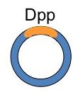
- In the early Drosophila embryo, the protein Dpp gets concentrated
in the dorsal most part of the embryo and plays a role in dorsoventral
patterning there. The system could be considered a closed ring. Could
a similar mechanism theoretically define the position of the peak in
this circular system (does the model still produce a more or less
stable peak under periodic boundary conditions)?
Submit the program
Thanks to Hans Meinhardt for providing materials!